Notes on ML
RAG
I have built a basic RAG. It was terrible. So I am going to start over learn from https://olickel.com/retrieval-augmented-research-1-basics Make a couple of notes and note down how to make it better. I want to be able to do RAG on any data(code, documentation whatever)
LLMs: Limited by the knowledge cutoff and context length limitations. RAG: LLM + data they have never seen before -> good results Most RAG pipelines: Import information + Embed results + retrieve relevant chunks to the question + import these chunks to the limited context of the model and ask it to answer the question
retrieve relevant chunks to the question : the hard part. Retrieving the relevant documents just by understanding the question is a pretty tall order. As complexity of question increases the way you retrieve relevant information will differ.
Embeddings and Embeddings model:
“Relatively low dimensional space onto which you can translate high dimensional vectors. Embeddings make it easier to do ML on large inputs like sparse vectors representing words. Embedding captures some of the semantics of the inputs by placing things that are similar closer in space.”
Embeddings: sentences with similar concepts cluster together, even if none of the text looks the same. Think embeddings think similarity. Different models must store and process the info differently so the embeddings of one might be directly comparable to other models embeddings.
Traditional methods: BM25 and TFIDF rely more on text similarity and less intelligent than ML based embedding based retrieval. They are mostly inscrutable we don’t fully understand it and sometimes doesn’t work, hard to debug. But they are less brittle and more closer to how brains work.
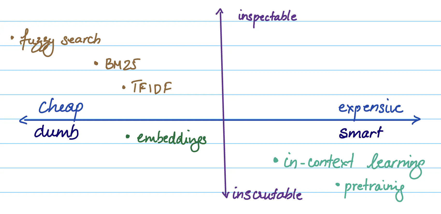
Question complexity:
- Single fact retrieval: “what is xxx?”
- Multi fact retrieval: “what are all the ways to do x?”
- Discontiguous multi fact retrieval : information Is not continuously present in the source. “What are all the ways discussed in article to build x?”
- Simple analysis: requires understanding of one section of document. “What is the main part of this article? How do they x?”
- Complex analysis: Harder questions and require extended information from multiple parts of a dataset. “How does x compare to x?”
- Finally research level analysis: “Why is this outside the scope of this? When will this hit a ceiling according to the arguments and limitations here?”
You need to understand the complexity to build a better RAG for sure. I think the goal with any intelligent system you want to build should be to make it less black boxes. You can use many methods to do so. But the goal should be to do that.
Single shot is not good enough: It’s not how you process information so how can LLM process information that way. Moreover expecting single shot RAG to hit higher and higher benchmark is placing an impossible requirement of intelligence purely on the Retrieval system. You can make the LLM the big brains to improve the pipeline dramatically, make it ask for more information and use this information for multiple rounds of retrieval.
Steps for multiple shot retrieval
- We need to extract partial information from retrieved pieces of stored data, so we can learn as we go.
- We need to find new places to look, informed by source data as well as by question.
- We need to retrieve info from those specific places.
This is what walking GPT is doing basically. I don’t know, I need to implement this to figure out what the heck he is talking about Multi turn retrieval:
- Fact extraction:
- Finding new threads
- Connecting threads
Plain text is your friend, remember that embeddings is fuzzy, the way you use it can make it ultimately into a terrible messy search. So the first step in the pipeline should be to extract the right source of information from your source document before you do any sort of chunking etc.,
Summarisation, tagging classification by LLM can all help you in this.
Reducing the distance between the question you are asking and the source document. Use LLMs as transformation tools before doing RAG that’s the summary.
Okay the best thing I got out of it is you can make RAG is just experimenting and you can make it truly complex and also terrible, like no way to determine which.. or is there.
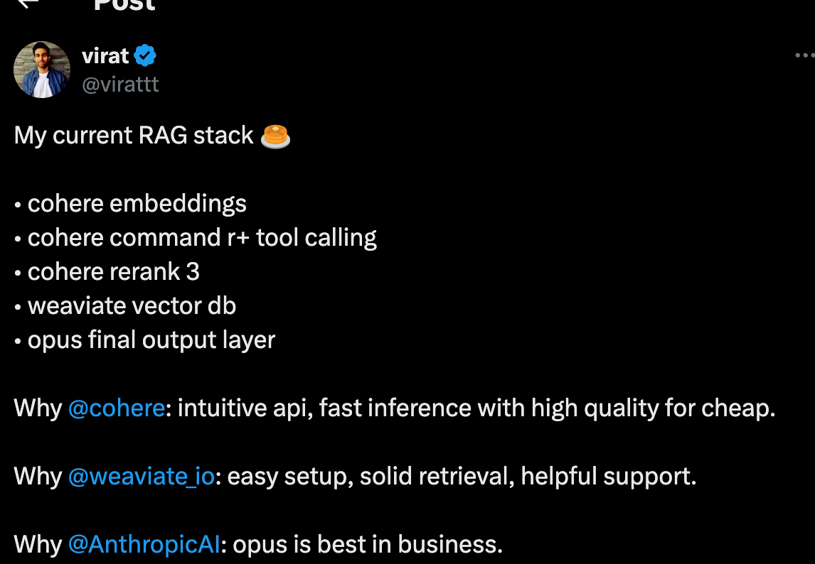
Code RAG
Reading material: https://sankalp1999.notion.site/Learnings-from-codeQA-Part-1-5eb12ceb948040789d0a0aca1ac23329
Problem statement
- Ask questions about codebase in any language -> get answers for it.
- Should provide relevant code snippets
- Should know the classes, references or any structures that are defined in the code.
- This can then be used to help get answers to how to change the code to achieve some other task
Questions can be simple->single hop or complex->multi-hop To an extent be able to handle uncertainty in the method name or any reference name that you use in the question. It’s a natural language query and you can ask random questions.
Discussion
In context learning approach: LLM have good context length now. But like cursor or copilot can’t do that. Like no don’t want to copy my code and find reference to write my code. Also most production codebases are huge and copying all the code in context won’t work. There is always a limit. So we will use RAG to basically simulate this copy pasting.
Extracting relevant code for the given question
We need Semantic Search (basically search based on meaning and context of the query and not keyword search) We do this code search with embeddings. Basically think of it as a dense vector representation of the data that you have. These embeddings will capture the semantic meaning of the code base in a high dimensional space. Some common embedding techniques include word embeddings (e.g., Word2Vec, GloVe), sentence embeddings (e.g., BERT, RoBERTa), and document embeddings (e.g., Doc2Vec). Word embedding: Represent word in a vector space. The main idea behind word embeddings is to capture the semantic and syntactic relationships between words based on their co-occurrence patterns in a large text corpus. Ex: word2Vec Sentence embedding: Extends concept of word to sentence or like a chunk of text or group of words in a way. Ex: BERT, Roberts Document Embedding: Represent entire documents as dense vectors. Applications mostly in things like document similarity and such. It’s basically an extension of word2Vec again. #TODO: Read more about Word2Vec and BERT #TODO: Read nominic ai’s new embedding for multi-modal data. Try to use it for some database within 250K]
Basically the query will also be converted into the same vector representation and you will do a semantic search.
Chunking: [TBC]
Mastering LLMs notes
Fine-Tuning Workshop 1: When and Why to Fine-Tune an LLM
- Do not start with fine-tuning. Prompt engineering first.
- Write tests and assertions
- Ship fast
- Then if needed do the fine-tuning
Evals are central
What is Finetuning? You take sets of inputs and outputs and we train the base model. The trick to do this is use some sort of template. Here’s the input some tokens in between and then the answer
Example:
What is x?###X is blah blah.
Need consistent templating b/w training and inference.
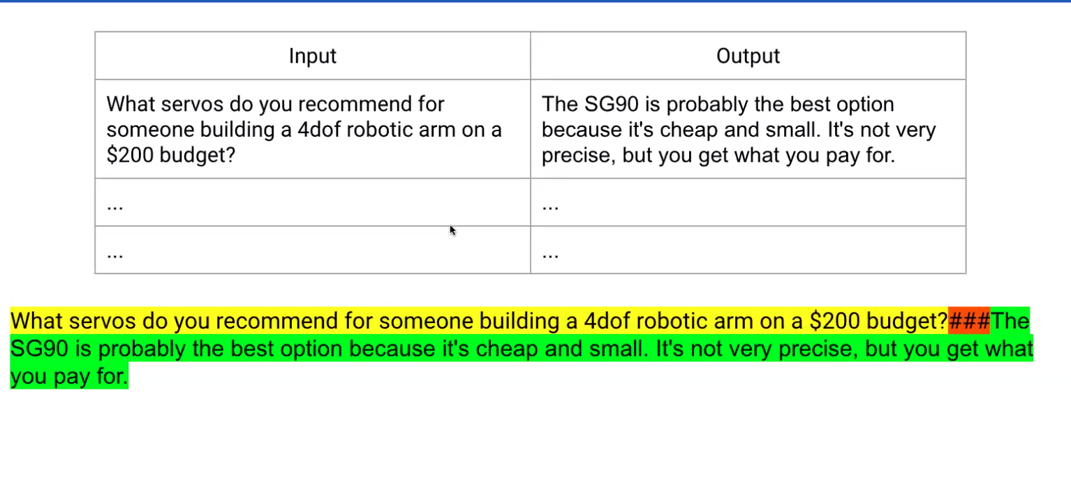
Important:
I.e, if you trained using ### b/w input and output, then you need to use the same token to differentiate at inference time too. Very important to understand template. Will coming back to this when learning axolotl. (Another template hugging face applied chat template method.)
Is finetuning dead?
- Niche cases
- If you don’t want to expose your data and sort of want your own model But in any case you should really prove to yourself that fine-tuning is necessary.
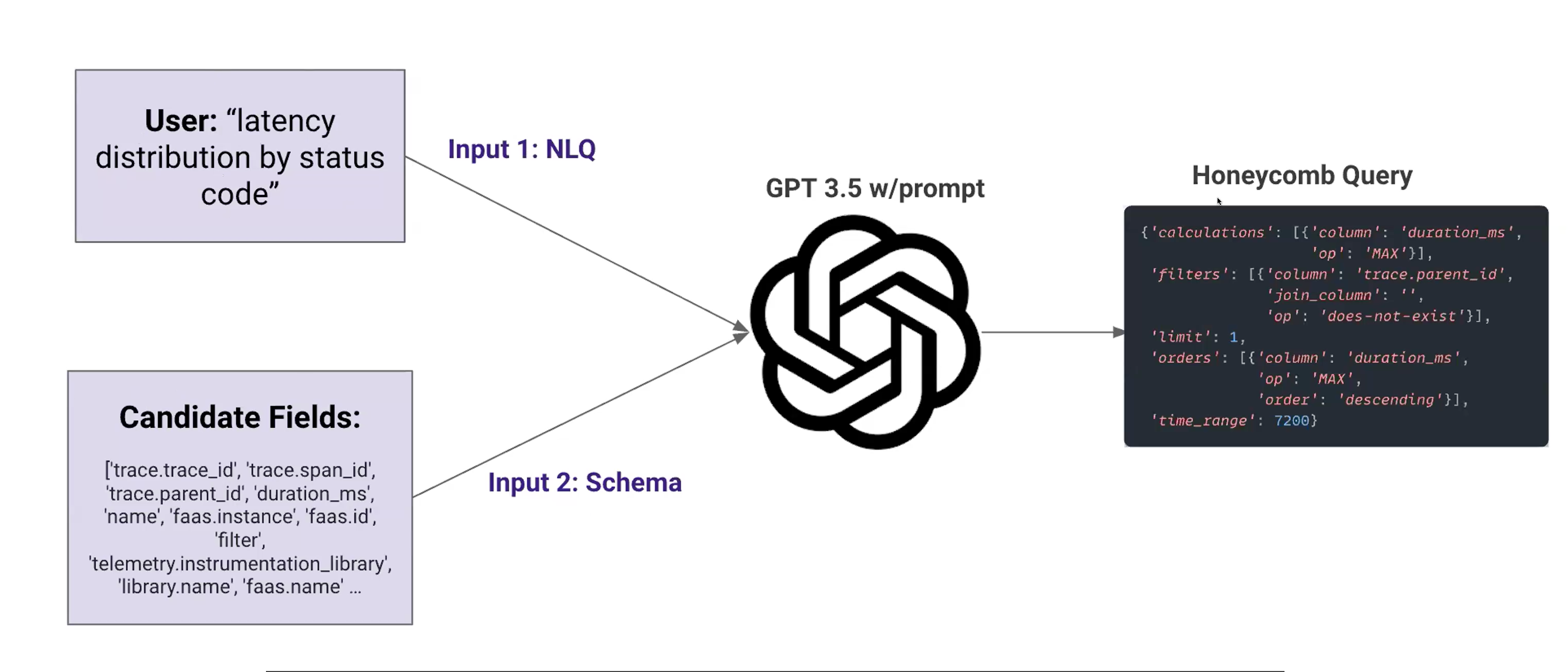
Case study: Honeycomb - NL to query Observability, Meet Natural language querying with query assistant. Basically like a natural language query to a honeycomb query(they have their own special DSL) Iteration 1: They basically used a query and a sort of RAG to get schema -> prompt -> get 3.5 and out comes a honeycomb query.
Reasons to fine-tune:
- Data privacy
- Quality vs latency tradeoff
- Extremely narrow problem
- Prompt engineering is impractical
Result: Fine-tuned model was faster, more compliant and higher quality vs GPT 3.5
- Should we do fine-tuning or RAG? If you fine-tune a model you want to fine tune it in such a way that it does better with RAG.
- Can you fine-tune a model such that it is better at function calling? Yes. And also need to find good examples to fine tune
- How much data to successfully fine tune? Least is like as low as 100. Depends on the scope of the problem you are dealing with.
- Is there value in fine-tuning on correct and incorrect examples? Later discussions to come on right vs wrong to preferring better and worse option.
- Multimodal finetuning LLAVA model is very very good at fine-tuning for multimodal fine-tuning.
- Generating synthetic data for fine-tuning Usually use the most powerful model to generate this synthetic data.
- Base model vs instruction tuned models Usually base model when possible. If it’s especially a very narrow use case. You don’t want to have to use a prompt at all. The sweet spot is to fintune a 7B parameter model. But there are some usecases where it’s too narrow.
Exercise: Imagine you decide to build a chatbot for your first fine tune project. What factors determine whether fine-tuning a chatbot will work well or not?
My answer:
- What purpose does the chatbot serve? Will the user expected inputs be widely scoped or not?
- Is there good data available for finetuning. Wide scope: needs immense amount of data.
- Will few shot work? Is it just a matter of format and there is not a lot of specialised data/context.
- Is it language finetuning etc., in that case finetuning works very well.
When someone asks you to make a chatbot:
- Manage user expectations: can’t really make chatbot that makes everything. Its AGI. Not really the best user interface.
- Large surface area
- Combination of tools
- Compromise-specificity
Guardrails: Most of them bad. Mostly don’t work. They just use prompt really.
When to fine-tune? Recap
- Want bespoke behaviour
- Valuable enough to justify operational complexity
- Have examples of desired input/output
Preference optimisation:
DPO: Direct Preference optimisation. Supervised finetuning.

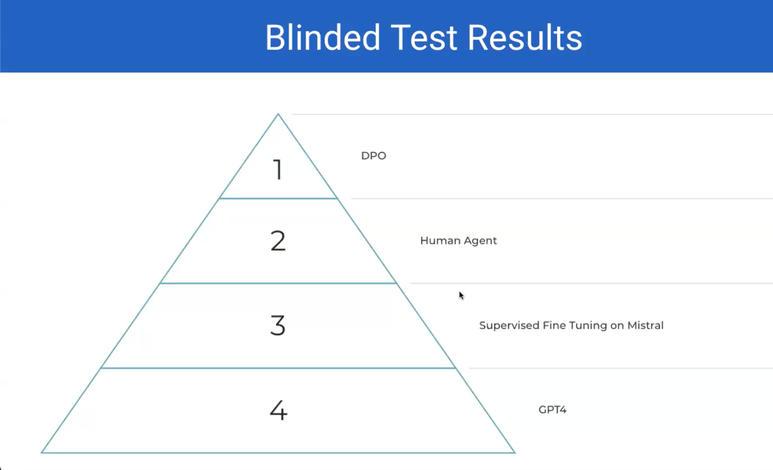
Finetuning some example given:
- Restaurant chain wants to create a email response customer bot > data probably available. The style is very hard to convey through prompt for sure.
- A medical publisher has an army of Analyst that classify each new research article into some complex ontology that they have built.
Few shot examples and fine-tuning.
Basically if there are some fixed things that you are using fine tuning should be able to take care of it. But if there some dynamic things that you want to add maybe few shot is good.
Recap: Philosophy:
- Start easy, step up the ladder of complexity slowly
- Shorten the development cycle
- What makes a good first product
Picking an LLM use case: List 5 LLM use cases you personally have or that you think are especially interesting
Describe each use case in 1-2 sentences Then write 1-2 sentences describing whether is is best served with fine-tuning, RAG, prompt engineering or some combination
Post ONE use case and the reasoning behind your approach in the course forum by May 21.
- Customer service chat bot for a food delivery service company: Good to fine-tune in case you have data already. There is a style element. Prompting is not possible(data privacy). I.e, need local model.
- Function calling models for agents: Improved accuracy large amount of data available. And the API call of some of these are fixed.
- Fan Fiction writer: You want to allow fans to create a sort of continuation or alternate ends to your story but it has to be written in your style. You can train on the data available. Do DPO etc., then better to use finetuning in this case.
#TODO: Read https://hamel.dev/notes/llm/finetuning/05_tokenizer_gotchas.html Your AI Product Needs Evals](https://hamel.dev/blog/posts/evals/) #TODO: Build a simple Regression model
Axolotl notes
What is it? A tool that helps you fine-tune a bunch of models and offers support for different configurations and architecture to do it. It took too much time to get axolotl to work on Mac. Ughh.
Mastering LLMs notes-2
Week 2 class 1: How to be successful with this:
- tinker with the tools we show you
- importance of blogging
- how to share your work- blogs, projects, etc.,
Model choices:
- What base model to fine tune of?
- 7B and 13 B are the most popular to fin tune.
- which model family to use?
- thanks to axolotl its extremely easy to fine tune a bunch of different models and just experiment.
- Should you use LORA vs full fine tune?
- Lora in a nutshell
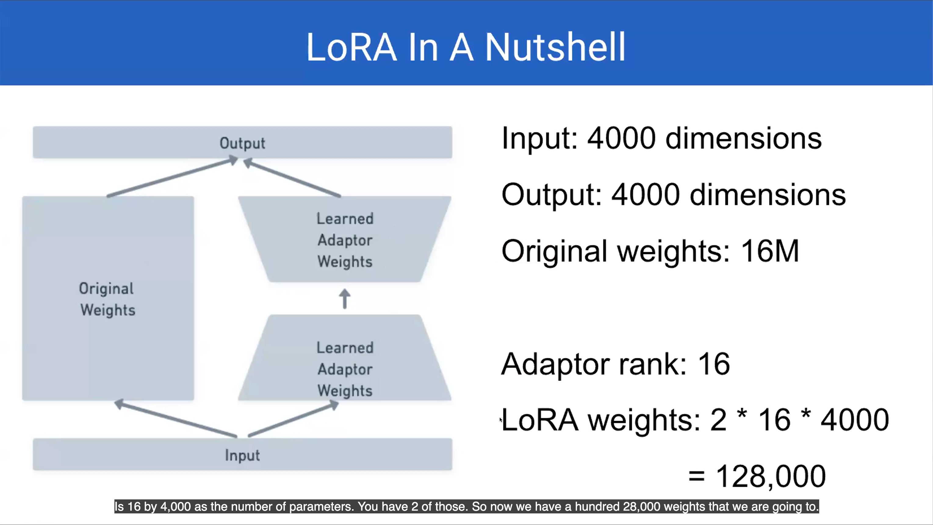
So using this requires as you see a lot less RAM. 16M vs 128000
QLora: Lora at lower precision. Memory savings with possible loss in quality. #TODO: Learn the details behind LoRa and QLoRa
What is axolotl:
- Wrapper for hugging face tools
- Ease of use. Focus on data
- Built on best practises
Using axolotl
The example configs are super helpful and also all the commands-> preprocess data -> fine-tune the model -> inference.. are all there in the GitHub readme file.
Even though your data looks like this…
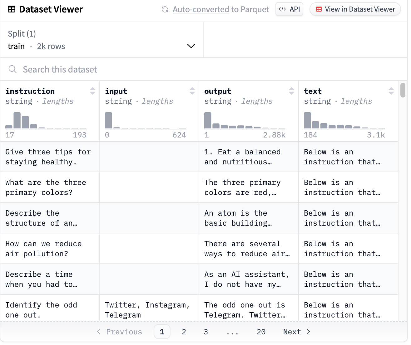
Your model is going to train on a string. Basically the template for that string is something like:
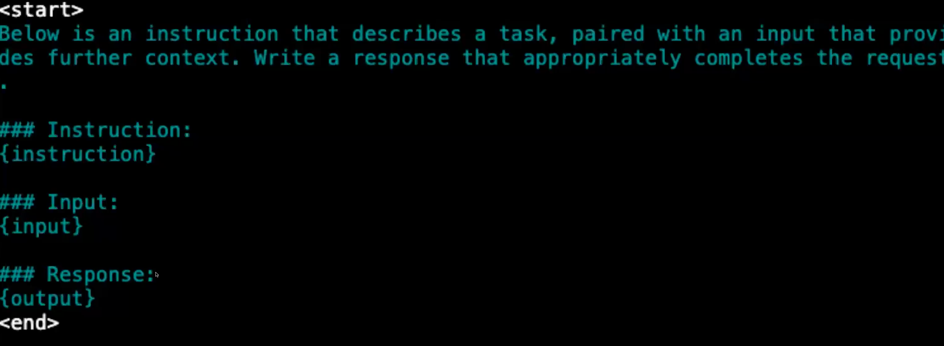
The preprocessing step will basically create strings that you are going to train on. At inference you use the same template. Every thing upto response basically.
One more important thing is Masking. So most training we want to train the model to generate like on the output so we use a mask to sort of tell the model that (#TODO: Learn more about the masking for training data)

Case study:
Honeycomb - NL to query
Problem statement
All the code for this is here: Sushmithamallesh/ftcourse
- You should write evals
- Level1: Unit test. Mainly assertions .. is the json valid, are columns valid, basically is model doing the right thing. He mostly wrote pytests.
- You have to clean your data. Use assertions for this too. Assertions are not just for tests also for cleaning data.
Generating synthetic data
- There is no hard and fast rule about how much data you need.
- Sometimes good results come with 1000 examples even.
- Have to keep a separate eval set data too
Basically the prompt you would use incase the model wasn’t fine-tuned. The prompt with all the info about column names, and the whole context, is to be repurposed to create the synthetic data.
 Will the data created be junk? Duplicate? Yes. You need to use the assertions(level1) to clean out all this data.
Your JOB is to create and clean and look at assert that data is good
Prepare data for axolotl There are bunch of formats in axolotl. You need to use one of them. In this case they have used axolotl to use Axolotl - sharegpt format.
Basically make synthetic data -> clean that data(good level 1 assertions at least) -> organise data according to some axolotl template. -> preprocess data -> check and double check -> then train etc.,, -> then sanity check your model -> improve the data(in case the outputs are not upto mark)(can use many techniques like LLM Judge) -> Curate the data
Different things to try while doing the training itself
- Varying learning rates
- Learning rate schedulers
- Distributed schemes(Deepspeed Stage Zero/Three)
- Batch Sizes
- Sample packing vs Not Sample Packing Choose the best model according to eval loss. Sanity checking model Local inference: You need to generate predictions so you can test the model. There are bunch of ways you can make the data better given you figure out the model created data is bad. One such example he explains is creating a model that is a critique of the data that gets generated. He used a human to write critiques. And then trained the llm to be as good a critique as the human. Then used this critique when generating the data to get out better data. Basically this is just one good way, one tool in your box. Can be many many others.
Once you curate? Should you fine tune the fine-tuned model or the original model from scratch. Ans: Always mostly from scratch. Otherwise overfitting.
Scaling model training with more compute, How do they do it? (By Zach mueller)
- We can somewhat estimate the memory usage in vanilla fine tuning
- Some assumptions:
- Adam optimiser
- Batch size of 1 Back of the hand calculation:
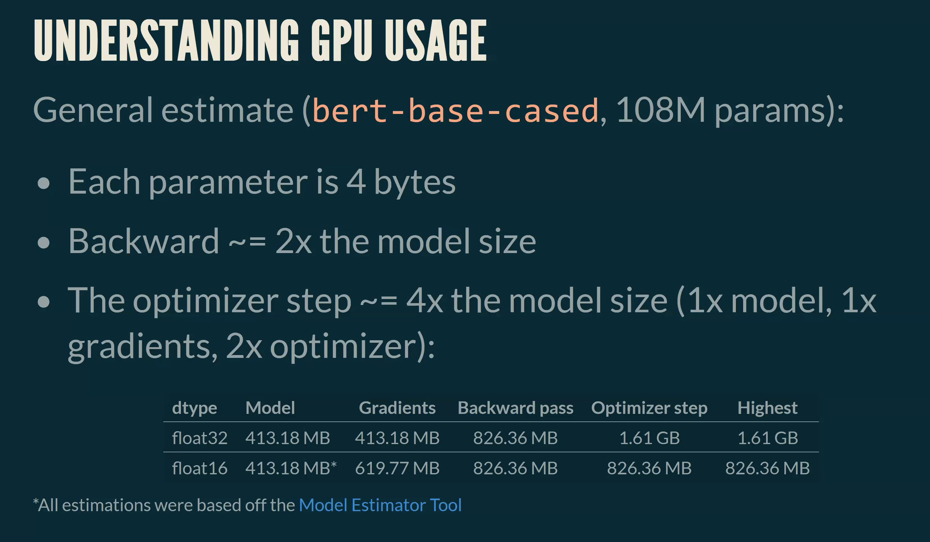
In the above figure calculation is for batch size of 1. the second row in the table is with mixed precision.
This works for small models but if you do the same calculation for large models, it’s a huge huge difference.

Distributed training
Kinds of training:
- Single GPU
- No distributed techniques at play
- Distributed Data Parallelism (DDP):
- A full copy of the model exists on each device, but data is chunked b/w GPUs
- Fully Sharded Data Parallelism(FSDP) and DeepSpeed(DS):
- Split chunks of the model and optimiser states across GPUs, allowing for training bigger models on smaller(multiple) GPUs
Fully Sharded Data Parallelism
Basically we take a full model and we create shards of the model.
PEFT: PEFT stands for “Parameter-Efficient Fine-Tuning.” It refers to a set of techniques and approaches aimed at fine-tuning large pre-trained language models, like GPT-3 or BERT, while minimizing the number of trainable parameters.
FSDP: Getting parameter specific
- Different parameters dictate how much memory if needed for total GPU training across multiple GPUs.
- These include how model weights are sharded, gradients and more Example: Full Fine-Tune of Llama-3-8B without PEFT on 2 x 4090’s taken when explaining
So the gist of it, the more shards there are the more communication overhead. Because the shards of the model still sorta have to communicate with each other.
sharing_strategy:
How do we split the memory?
Dictates the levels of divvying resources to perform:
- FULL_SHARD: Includes optimiser states, gradients and parameters
- SHARD_GRAD_OP: Includes optimiser states and gradients
- NO_SHARD: Normal DDP
- HYBRID_SHARD: Includes optimiser states, gradients, and parameters but each node has the full model
auto_wrap_policy:
How the models should be split? Can be TRANSFORMER_BASED_WRAP or SIZE_BASED_WRAP: The first is specific to transformer. Can choose the layer you want to split on like Bert layer or llama layer etc., The latter is more manual. Just saying like after x amount of parameters go ahead and split the model.
offload_params:
Offload parameters and gradients to the CPU if they can’t fit into memory. This allows you to train much larger models locally, but will be much slower
Hugging face accelerate
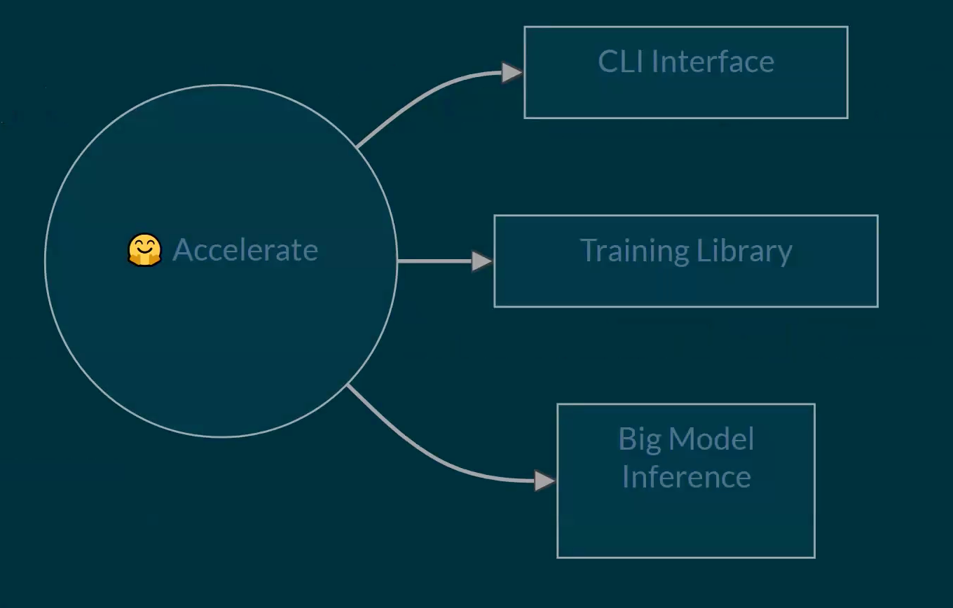
Basically to launch a distributed training: accelerate launch script.py
You can go through the config.yaml file and modify it as per your needs
How accelerate scaling works?
- Works off a sharing mindset. We split/shard the data across n nodes(GPUs) instead of sharing the same data across n nodes
- This speeds up training linearly
- Given a batch size of 16 on a single GPU. If we have 8 GPUs then we have 2 batch size on each of these
- This also means scheduler will be stepped n GPUs at a time per global step.
Key takeaways:
- You can scale out training with accelerate, FSDP and DeepSpeed across multiple GPUs to train bigger models
Modal: Basically a platform to run your model remote super well. Some useful links: llm-finetuning/nbs/inspect_data.ipynb at main · modal-labs/llm-finetuning
Conference talk pointers: Kyle Corbitt
First rule of deploying fine tuned model in production. You shouldn’t if you already have a really good pipeline that is already working. Just use prompting or additionally few shot RAG etc.,
Unless: You can’t hit the quality or latency target or cost target
Second rule: You should still write a prompt that gets you really good results. This creates baseline to compare to and prove the task is possible.
Works with prompting? 90 percent chance fine-tuning makes it better
Doesn’t work with prompting? 25 percent chance fine-tune won’t work at all
0 —GPT-4—>1 —Fine-tuned model—>100
Third rule: Review data. Go through some sample of data. Learn to use tools to understand the data. Ex: open pipe
Fourth rule: You will actually use the data. Example lot of people reject the bad prompt-response, by simply rejecting it as bad data, and just dropping it. But it might turn out that there is a quirk in the input that is actually a real input and your model might do a bad job on that later. So manually review data.
Make sure the data coverage is correct. According to him sometimes the data if its wrong here and there like 10 percent it really doesn’t matter that much. You can still get great results.
Sixth rule: Before training, have to pull out a test set. Grab 5-10 % of data in random. Very important.
Fifth rule: Choosing an appropriate model.
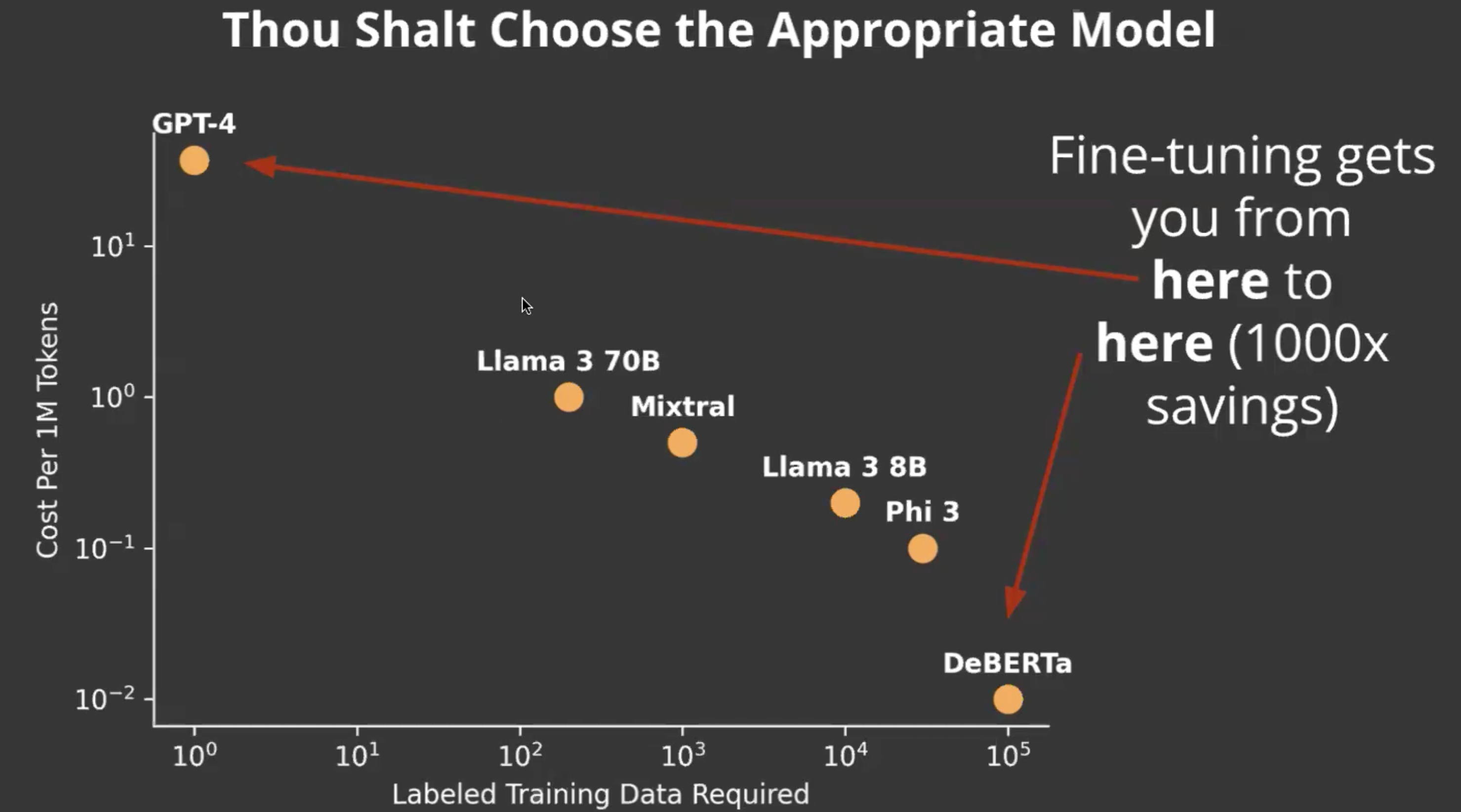
Seventh rule: Write evals. Write Fast evals. Two different kind of evaluations: Fast evaluation: That you can run in your training loop, even if you are doing prompt engineering(should be relatively fast). A good sweet spot for this: is using the LLM judge. For specific tasks like classification there might be different ways, but in general the point is write good fast evals and use them to iterate fast.
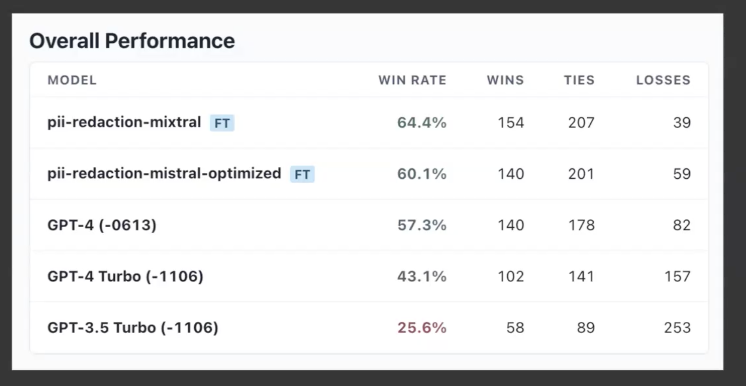
Eight rule: Write slow evals. This is the ultimate test. There is no one set rule on what tests these should be, but they are very important and should cover what your product direction is.
Ninth rule: You should not fire and forget. Something is going to change about the world, product direction etc., over time your model might not be as well adopted so you need to have a process for evaluating your model continuously.
Tenth rule: Don’t take any of these rules seriously. Understand the data, model and develop intuitions
Intuition for when to fine-tune. The more specific your task, it’s a better idea to fine-tune.
Lora vs QLora: Not a lot of fine-tune difference. Dora apparently is as good as full fine-tune performance. Start with Lora see if it gets you where you want, then do full fine-tune or Dora.
Office hours: Wing Lian Pointers
- Axolotl also supports template free prompting
- To go through data templates and experiment a bunch
Office hours: Zach Mueller
- Advice on getting better: Just train models, tweak, experiment, play
- Messing around -> write it down -> science
Notes for Attention is all you need
Transduction models: Basically models that take an input sequence and produce an output sequence. Both input and output sequence can be of varying lengths. Key points:
- Both of the input and output are a sequence.
- Models are mapping from one sequence space to another.
- Example: translation, summarisation, speech recognition, Question answering
- Example models: Seq2Seq models, Transformers, LSTM networks when used for sequence mapping
- Anti examples: Classification models, régression models,
So typically RNN works like this to process an input:
- Sequential processing in RNNs: They operate on one symbol at a time, in order. Each step produces a hidden state(ht) based on previous hidden state(h t-1) and current input.
- Alignment of positions with computation time: Each position in the sequence corresponds to a step in the computation. Model processes sequence in order from start to finish.
- Limitations on parallelisation: each step depends on previous one, not possible to process different parts of the sequence in parallel with a single example.
- Impact on efficiency: Limitation becomes problematic for long sequences. As sequence gets longer, time to process increases linearly.
Bottleneck in RNNs: Inability to parallelise within a sequence. Leads to:
- Slower training times
- Slower inference
- Difficulty with long range dependencies
Attention mechanism existed before this paper, but it was mostly used in addition to/as part of RNNs. But this paper proposed a new transformer architecture that basically relied mainly on attention mechanism. It allows for more parallelisation.
Background:
CNNs can do parallelisation and this has been used to optimise in case of models like Bytenet, ConvS2S. These models compete hidden representations in parallel for all input and output positions. This is in contrast to RNNs where everything happens in sequence.
Tradeoff: While these models allow for more parallelisation, they introduce a different challenge: number of operations required to relate signals from two arbitrary position grows as distance b/w these positions grow. Basically they trade off the computation problem of RNNs for a different problem - capturing the long-range dependencies efficiently.
TLDR: RNNs have parallelisation issue and CNNs have long range dependency issue. Transformers this is reduced to a constant number.
Self attention:
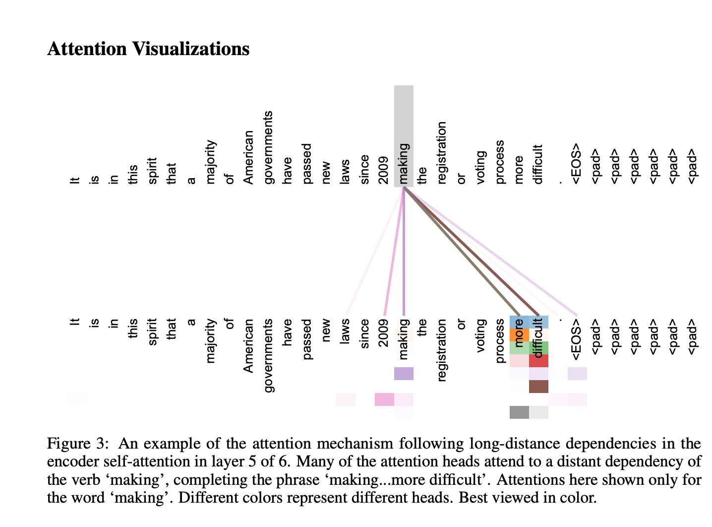
Self attention is a mechanism which allows a model to focus on different parts of the input sequence when processing each element of that same sequence. Also called intra attention. Contrast with traditional attention: Traditional attention works with two different sequences (I.e, machine translation, attention b/w source and target). Self attention operates within a single sequence.
TLDR: Self attention captures the spatial representation of the input sequence itself. CNNs also do that but in a different way. In CNN it’s sort of like a fixed-size, sliding scale, so the spatial relationship captured is sort of local. So its better for images, time series captures etc., Self attention captures this relationship regardless of distance, lets see in the next parts how.
End-to-End memory networks
These are neural networks designed to read from and write to a kind of external memory. Key features:
- They use attention mechanism to access this memory.
- They can be trained end-to-end meaning input to output without rewiring hand drawn intermediate steps.
- How they work?
- Input: They receive input
- Memory: They have “memory” component that stores information
- Attention: They use attention to find relevant information from the memory
- Output: They produce an output based on the input and retrieved memory.
- Difference from RNNs: RNNs process data sequentially. So no memory other than previously computed.
- Recurrent attention: They apply attention multiple times. This allows network to reason over multiple steps refining its understanding. Transformers do not use End to End networks, but they rely on attention mechanism to achieve this sort of thing.
Model architecture
In a traditional architecture of encoder-decoder: encoder maps an input sequence of symbols (x1, …. Xn) to a sequence of continuous representation z = (z1…. Zn). Given z decoder generated output (y1… yn) one at a time.
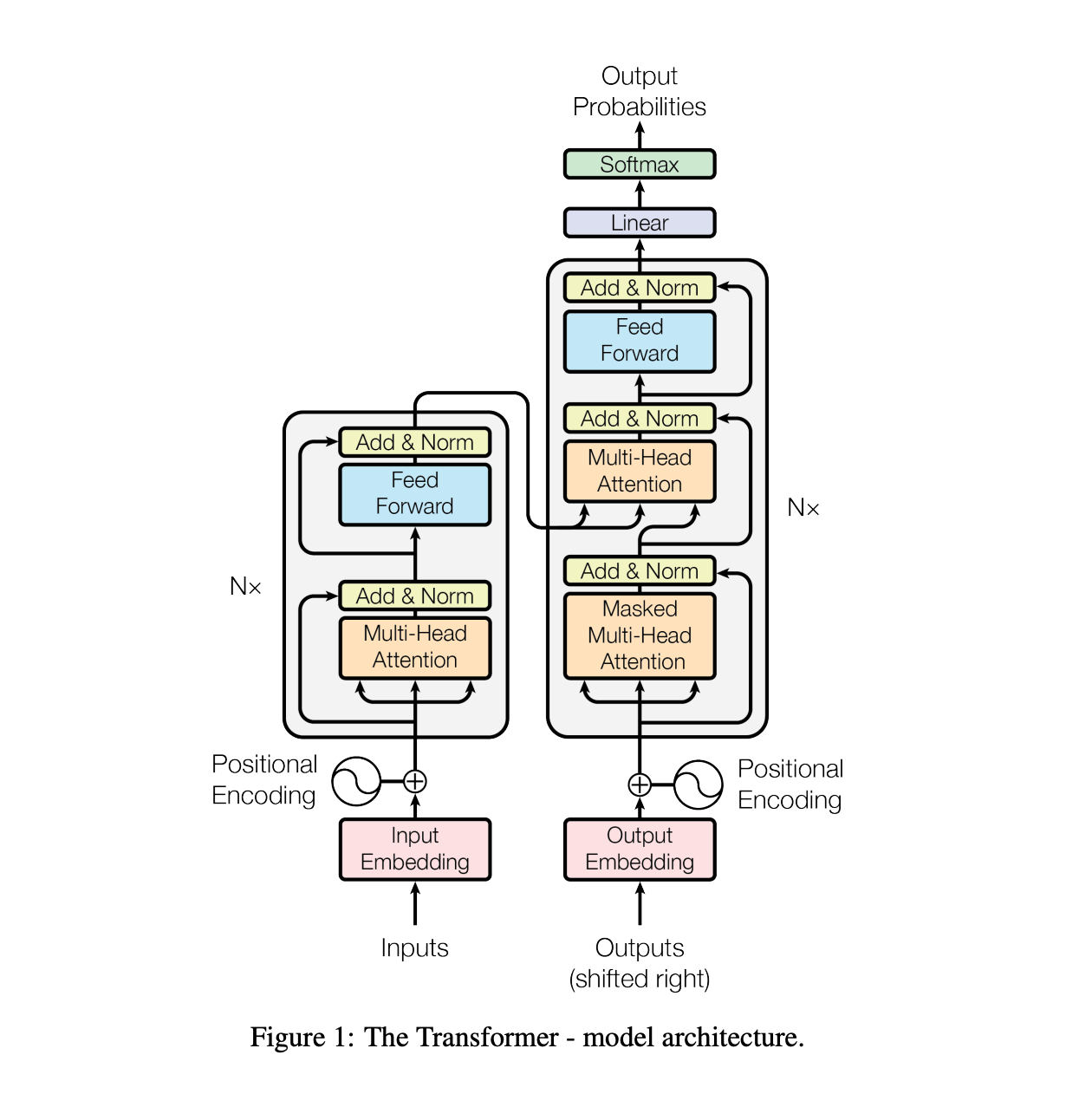 This is the architecture that the transformer follows using stacked self-attention and point-wise, fully connected layers for both encoder and decoder.
Autoregressive models:
Autoregressive means that the model generates output sequentially, using its own previous outputs as inputs for generating the next output.
In Transformer decoders:
- The decoder takes the encoder output and the previously generated tokens as input
- It uses self-attention to consider all previous outputs when generating the next token
Step-by-step example: Let’s say the model is generating a sentence:
- It generates the first word based on the input/context
- It generates the second word based on the input/context AND the first word it just generated
- It generates the third word based on the input/context AND the first two words it generated
- This process continues until the sequence is complete
Multi head self attention
Self attention: Allows the model to focus on different parts of the input sequence when processing each element. Each element can attend to other elements in the same sequence. Multi head: Instead of performing attention once. It’s performed in parallel. Multiple parallel attention operations.
How it works? Input is projected in three different representations: - Queries(Q) - Keys(K) - Values(V) Projection is done multiple times. Each head performs its own attention calculation. Results from all head are concatenated and linearly transformed.
Analogy: Imagine reading different parts of a sentences, different aspects of it(grammar, tone) and then combining all the aspects.
Masked multi head self attention
Basically the same multi head self attention but here we will have masked the input(at i) after i. This is basically to train the model to do next token prediction. During training the entire sequence is available but we will still mask the next tokens to ensure we do the training. During inference we allow the model to generate a token at a time. This is a decoder layer in transformers. Encoder needs to understand the full input so it uses multi head self attention, decoder needs to only see the previous outputs without peeking at future tokens. Encoder has another layer of multi head attention over encoder outputs after this.
Position-wise feed-forward network
It’s a simple layer applied to each position separately and identically. Components a) Two linear transformations b) A ReLU activation layer between them. This layer in there in both encoder and decode after the attention layer. Its basic functionality is to enhance the models ability to transform representation at each position. It complements the attention mechanism by adding another level of processing.
Residual connection
Residual connections also known as skip connections or shortcuts connections allow model to bypass one or more layers. Purpose: Helps in training very deep networks. It mitigates the vanishing gradient problem. It allows the model to access low level features. The output of each sub layer is added to its input .This sum becomes the input for next sublayer. Instead of passing the output of one layer to another, a skip connection added the input of a layer to its output. Basically it allows information to flow easily through the network.
Layer normalisation
This is a technique to normalise input across the features, typically applied to the activations of a layer. Applied after each layer after the residual connection layer. Layer norm unlike batch norm normalises across layers or features and not across batch.
⠀Important Takeaways: 1 The architecture is highly modular and repetitive. 2 It relies heavily on attention mechanisms, especially self-attention. 3 It uses techniques like residual connections and layer normalisation to facilitate training. 4 The decoder is designed to work autoregressively, generating one output at a time.
⠀This architecture allows the Transformer to process input sequences in parallel (unlike RNNs) while still capturing complex dependencies between different parts of the sequence. The multi-head attention mechanisms are key to its ability to focus on different aspects of the input simultaneously.
Encoder and decoder stacks
Let’s break down the key points to understand: 1 Overall Structure: * Both encoder and decoder consist of 6 identical layers stacked on top of each other. * This stacking allows the model to process information at different levels of abstraction. 2 Encoder Layer Components: a) Multi-head self-attention mechanism b) Position-wise feed-forward network * These components allow the model to capture complex relationships in the input. 3 Decoder Layer Components: a) Masked multi-head self-attention mechanism b) Multi-head attention over encoder output c) Position-wise feed-forward network * The additional attention layer allows the decoder to focus on relevant parts of the input when generating output. 4 Residual Connections: * Used around each sub-layer * Helps in training deep networks by allowing gradients to flow more easily 5 Layer Normalisation: * Applied after each sub-layer * Stabilises the learning process 6 Consistent Dimensionality: * All sub-layers and embedding layers produce outputs of dimension 512 * This consistency facilitates the residual connections 7 Masked Self-Attention in Decoder: * Prevents positions from attending to subsequent positions * Ensures the model doesn’t “look into the future” when generating sequences 8 Output Embedding Offset: * Decoder output embeddings are offset by one position * This, combined with masking, ensures the model’s autoregressive property
⠀Important Takeaways: 1 The architecture is highly modular and repetitive. 2 It relies heavily on attention mechanisms, especially self-attention. 3 It uses techniques like residual connections and layer normalisation to facilitate training. 4 The decoder is designed to work auto-regressively, generating one output at a time.
⠀This architecture allows the Transformer to process input sequences in parallel (unlike RNNs) while still capturing complex dependencies between different parts of the sequence. The multi-head attention mechanisms are key to its ability to focus on different aspects of the input simultaneously.
Attention
Basically attention is a transform mechanism to transform Query, Key and Values to output,
Components:
- Query(Q): A vector representing the current position or item we are focusing on
- Keys(K): A set of vectors representing all positions in the input
- Values(V): A set of vectors containing the actual content at each position
Process
- Compatibility: Calculate how well the query matches each key
- Weighting: Convert these compatibility scores into weights
- Aggregation: Use these weights to create a weighted sum of the values Basically for each input token which is a query, we define the attention calculation for other token which are the Keys we use the values and create a weighted sum of those values. This is done several times with multi head attention mechanism.
Note: There is a lot more details in the paper which I will visit later. For now this is the extent of the information I need to digest
The first law of Complexodynamics
The question that this essay is trying to answer: why does “complexity” or “interestingness” of physical systems seem to increase with time and then hit a maximum and decrease, in contrast to the entropy, which of course increases monotonically? [This was asked in a conference by Sean carroll]
The author will draw from Kolmogorov complexity to try and deduce the answer for this.
First of all, What is Kolmogorov complexity? It measures the complexity of any object by the length of the shortest computer program that could describe it. How much simply can you describe the object without loosing information about it.
Why is this more interesting than entropy? While entropy only can capture order, Kolmogorov complexity kinda captures “interestingness” or complexity in a much better way. Perfect order is simple you can capture it easily but complete randomness is also simple(“generate random noise”) but there are more complex things in the middle like say “describe an organism”.
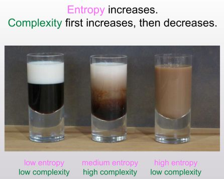
So this is what author wants to do: “
- Come up with a plausible formal definition of “complexity.”
- Prove that the “complexity,” so defined, is large at intermediate times in natural model systems, despite being close to zero at the initial time and close to zero at late times.
Not hard to explain why complexity is low in the beginning: Entropy is close to zero. Entropy is sort of an upper bound of complexity really. Not hard to explain the end: We reach a uniform equilibrium. At intermediate though: things are complex because the above constraints don’t hold. So how do we define this large complexity anyway? How high does it get anyway? How to measure it?
The author will use a notion called sophistication from Kolmogorov complexity to define this.
Using Kolmogorov complexity to define entropy Its not obvious as There’s a mismatch in deterministic systems:
- Entropy appears to increase rapidly (linear/polynomial)
- But Kolmogorov complexity only increases logarithmically (log(t))
- This is because you only need: initial state (constant) + time steps (log(t)) Solutions:
- Use probabilistic systems
- Use resource bounded Kolmogorov complexity:
- Add constraints like: time limit, limit of circuit depth, basically resource constraint - severe.
- Adding this sort of constraint increases the Kolmogorov complexity rapidly in sync with entropy and thus we use it to define it.
How can we define what Sean was calling “complexity”? [from the original quote from now on the author says he will call this “complexotropy”. [Backstory: Kolmogorov observed that what is seemingly complex like a random string is actually also least “complex” or “interesting” . Because you could easily describe it: it’s a random string that’s all it takes to describe it.
But how do we formalise the above intuition.(The sophistication bit actually”)
Given a set S of n-bit stings. K(S) -> number of bits in the shortest program to define this set S Given x an element of S: K(x|S) -> length of shortest program that outputs x given an oracle for testing membership in S. Sophistication of x of Sophistication(x) is the smallest possible value of K(S) over al the sets S such that
- x ∈ S
- K(x|S) >= log2(|S|) - c for some contant c.
Basically my understanding is we calculate sophistication by determining a possible K(S) that encompasses x such that the set S is not necessarily describing the randomness of x but still defining the complexity of it.
Some example: For the coffee cup above the set can be something like “a mixture of two liquids” it cannot be describing the swirls and the correct patterns in the mixture. So this set determines the sophistication of the x. S shouldn’t be too broad or narrow. Soph(x) is the length of the shortest computer program that defines not necessarily x but S of which x is a random member.
So sophistication seems to capture “complexotropy” well. It defines both simple string and random string to have low sophistication but defines middle to have high complexity Problem: But in deterministic systems
Same issue as earlier.
Can describe state at time t using just
- initial state
- transition rule
- time t
So sophistication is not above log(t) + c This is same for probabilistic state.
So sophistication doesn’t capture the intuition of “complexotropy” as well as intended. It doesn’t grow fast enough. We need to find some other way to measure this.
The fix: Constraint on computational resources. New definition: Any program that runs on n log n time. Then the above problem is solved for. So it’s not easy to just define the program by defining initial step and the time steps. Actually forces us to acknowledge the complexity there. Also this need not be *n log n *. It can be any time bound restriction or anything else.
The motivation is define a “complexotropy” measure that assigns a value close to 0 to the first cup and third cup, but large value to second cup. Thus we consider the length of the shortest computer program that not necessarily defines x but the probability distribution D such that x is no longer compressible in respect to D. (So basically x looks like any other ransom sample from D). Like think of the this as something similar to S but with time constraints. S vs D for my understanding: “D is a sophisticated S” S (Set):
- “All possible states of two mixing liquids”
- Just lists possible states
- No time constraint on generating them
⠀D (Distribution):
- “States you get when you actually mix liquids for t seconds”
- Some patterns more likely than others
- Must be able to generate similar patterns quickly
- Your specific cup should look like typical mixing at time t
The progression of ideas has been:
- Started with basic Kolmogorov complexity (wasn’t good enough)
- Moved to sophistication with set S (better, but still didn’t grow fast enough)
- Finally arrived at complexotropy with distribution D (adds requirements that make it work better)
The constraints should be imposed both at sampling program level. And at reconstruction algorithm level. Sampling algorithm: generate samples for D efficiently. otherwise Could just mention initial state, rules, time t Reconstruction algorithm: given a sample/pattern generate it efficiently. Given unlimited time can find x by finding special properties of x.
Together these two restrictions ensure we are defining “complexotropy” properly.
Notes: First of all it’s all conjecture. But it can be proved in some ways though. Two possible approach: Theoretical proof(author don’t know how). Empirical testing: simulate and use a system to prove it over time. Use approximation. Like gzip file size as proxy for complexity. Similar to using compression for Kolmogorov complexity
Conclusion
- The Core Question:
- Why do physical systems follow this pattern:
- Start simple (low complexity)
- Become complex (peak complexity)
- End simple again (low complexity)
- Why do physical systems follow this pattern:
- The Path to Answer:
- Can’t use entropy (only increases)
- Try Kolmogorov complexity (program length to generate x)
- Introduce sophistication (using sets S)
- Finally arrive at complextropy (using distribution D with constraints)
- Key Concepts:
- Sophistication: Measures structure without randomness
- Complextropy: Sophistication + two efficiency requirements:
- Must generate samples efficiently
- Must reconstruct specific state efficiently
- Important Requirements:
- Need resource constraints (like time limits)
- Need bounds on how specific/general our descriptions can be
- Without these, complexity doesn’t grow enough
- Practical Testing:
- Can use simplified models (2D pixel grid)
- Can use compression (like gzip) as approximation
- Still an open problem for rigorous mathematical proof
- Key Insight:
- Complexity isn’t just about randomness or order
- Most interesting complexity happens in between
- Like the middle coffee cup - not ordered, not random, but structured
⠀
Hamel: Your AI product needs evals
Your AI Product Needs Evals – Pointers:
- Unsuccessful LLM product have one common root cause according to the author: Failure to create a robust evaluation system.
- Iterating quickly == Success
Have processes and tools for
- Evaluating quality(ex: tests)
- Debugging issues(ex: logging and inspecting data)
- Changing the behaviour of the system(prompt engineering, fnnetungin, writing code)
You should focus on point 1 above.
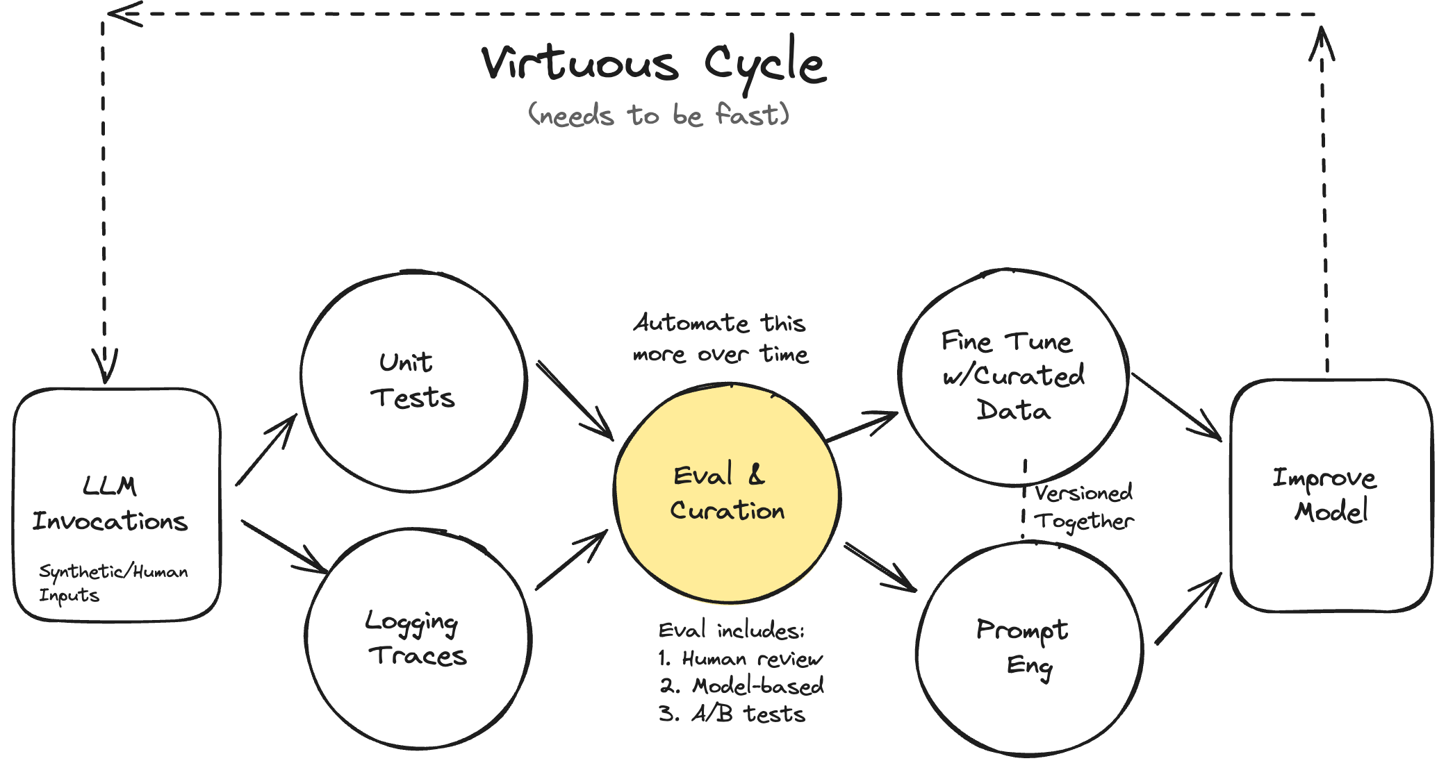
The types of evaluation
Level 1: Unit tests Level 2: Model and Human Eval(this includes debugging) Level 3: A/B testing
Cost of Level 3>Level 2 > Level 1 You can run level 1 on pretty much any change you make and then level 2 and 3 on significant product changes.
Level 1: Unit tests
Basically assertion tests. But it should not just be inference. You should keep them in places like data cleaning and automatic retries.
Step 1: Write scoped tests Break down the scope f your LLM into features it solves for and scenarios it will come across. The other thing is you need to test for some generic things. Like say is LLM exposing credentials that are meant to be private.
Step 2: Create Test cases Write test cases that will simulate there features you have listed. You can use LLM to generate these test cases synthetically.
You don’t have to wait for production to get these test cases. You can also use small set of customers to test first and get scenarios.
The more failures this way the better. You can improve your model later on learning from these failures.
You don’t need a 100 % pass rate like traditional tests. You need to make decision on the tolerance level of failure of your product.
Step 3: Run and track your test regularly
Use regular CI infrastructure in most cases. Use good visualisation for failure cases etc., Collect metrics well.
Level 2: Human and model eval
Prerequisite for this in a way similar is to log your traces.
Hamel likes Langsmith : ) for tracing
Look at your traces All friction from viewing data should be eased. You should have a data viewing tool and you need to gather all info necessary. It might be sometimes necessary to build a custom tool to achieve this too. Label data on a binary good or bad grade to then further use it for finetuning I guess
How much data do you have to look at? In the beginning at least as much as you can. Then you can start doing sampling and lessening the burden.
Level 3: A/B testing
Basically ensuring your model is driving user behaviour or outcomes you want.
Pointers:
- Remove all friction from looking at data
- Keep it simple. Don’t buy fancy LLM tools
- You have to be looking at lots and lots of data
- Don’t rely on generic evaluation frameworks to measure the quality of your AI. Create a specific solution to your problem.
- Write lots of tests Frequently update them.
- LLM can be used to unblock the eval system. Example use LLM to
- Generate test cases and write assertions
- Generate synthetic data
- Critique and label data
- Reuse your eval infra for debugging and fine-tuning